6.3 Plot
Por um escritor misterioso
Descrição

Section 6.3 - Curves Of Best Fit - ProProfs Quiz
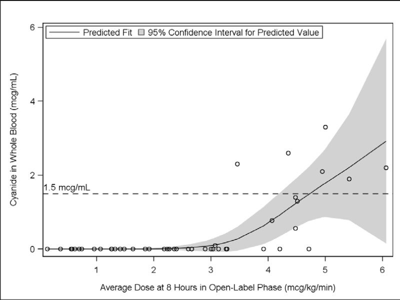
Figure 14.1.6.3, 8 Hour Dose Response Model of Cyanide and the AUC for Administered SNP Model for Cyanide=0: Logistic with Probability (1+exp(b0_p+b1_p*DOSE))−1 Model when Cyanide>0: Gamma with Mean exp(b0_g+b1_g*DOSE) - A Phase
6.3: Derivatives of inverse functions. - Mathematics LibreTexts

6.3. Fitting Data II — PHYS 27 Scientific Computing Tutorial 1 documentation
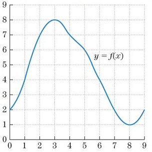
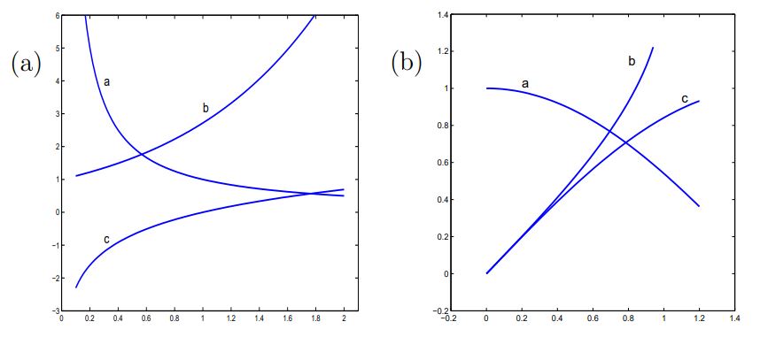
In Exercises 37 − 40 , use a Riemann sum to approximate the area under the graph of f ( x ) in the fig. 14 on the given interval, with selected

10-Year Treasury Yield Breakout Targeting 6.3 Percent? - See It Market
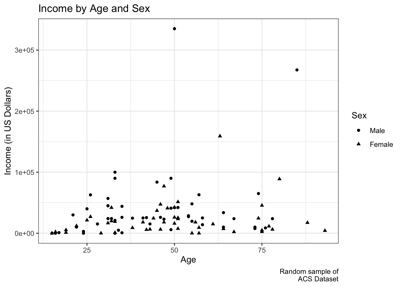
6 Customizing Plot Appearance Data Visualization in R with ggplot2
Understanding The Monte Carlo Method - by Nick M
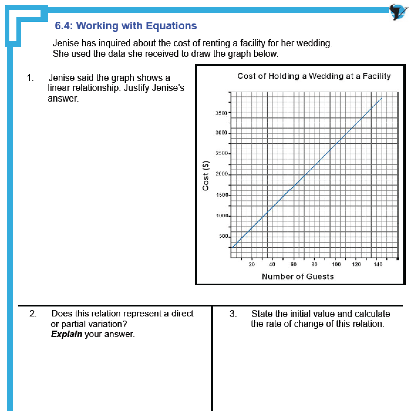
6.3 - Mathematical Models/Multiple Representations of Linear Relations

6.3 Plot
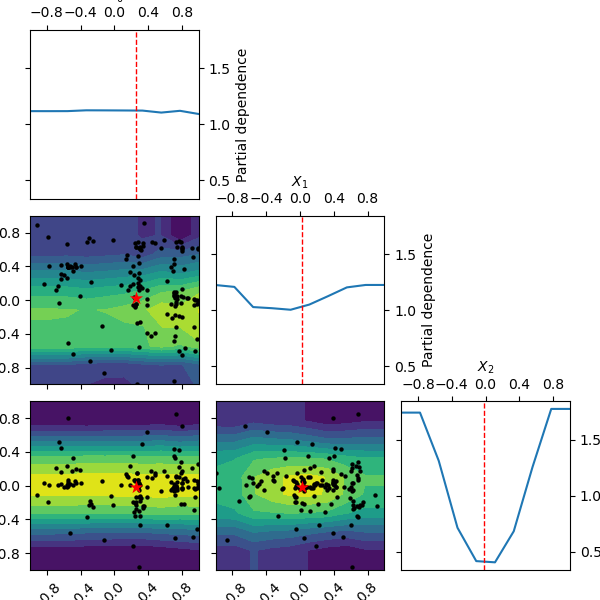
6. Plotting tools — scikit-optimize 0.8.1 documentation
Plotting your data

6.3 graph of sine, cosine and tangent functions - Flip eBook Pages 1-14
de
por adulto (o preço varia de acordo com o tamanho do grupo)